ResearchProbability explained
Why randomness creates streaks and clusters
Six heads in a row. Dots that bunch together. An Ace that never seems to arrive. The rules behind chance explain more than appearances do.
A fair coin lands heads six times. Your music shuffle repeats an artist. A scatter of dots has a conspicuous gap. Each result can feel less random than a neat mixture would.
But “random” describes how an outcome is produced. It does not promise a tidy-looking result. Independent choices can create runs and clusters; a process that deliberately spreads everything out follows a different rule.
The stock in Forty Thieves Solitaire reveals cards one at a time. That makes a useful contrast with a coin: drawing without replacement reduces a finite supply, while a flip does not use up a supply of heads or tails.
To make the distinction visible, we worked through three simple models: fair coin flips, uniformly placed points and a shuffled deck. The calculations below show what changes the odds—and what does not.
Six heads looks unusual. Its probability is not unique.
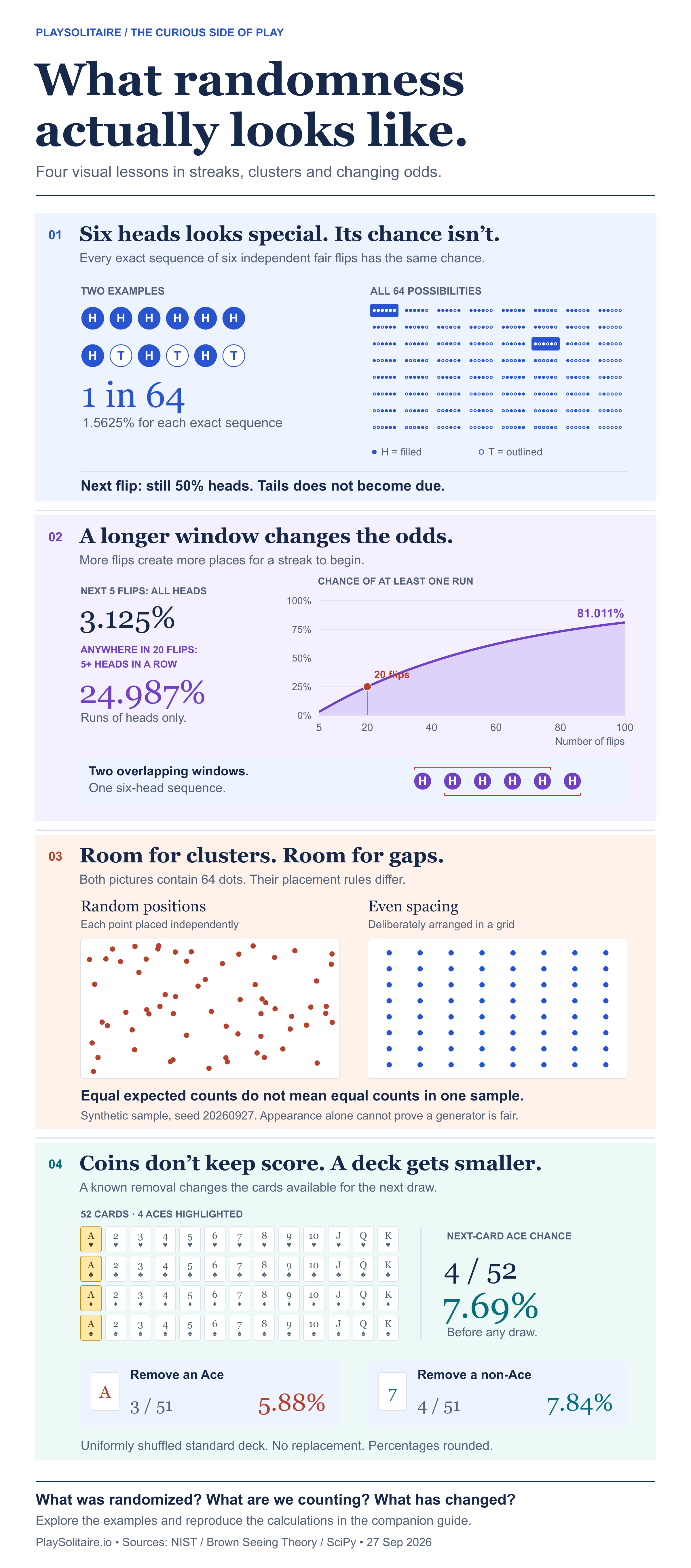
Compare two exact sequences: HHHHHH and HTHTHT. For a fair coin with independent flips, each has probability (½)⁶, or 1/64 = 1.5625%. The alternating sequence is just as specific as the run of heads.
Different patterns. The same chance.
1 in 641.5625%
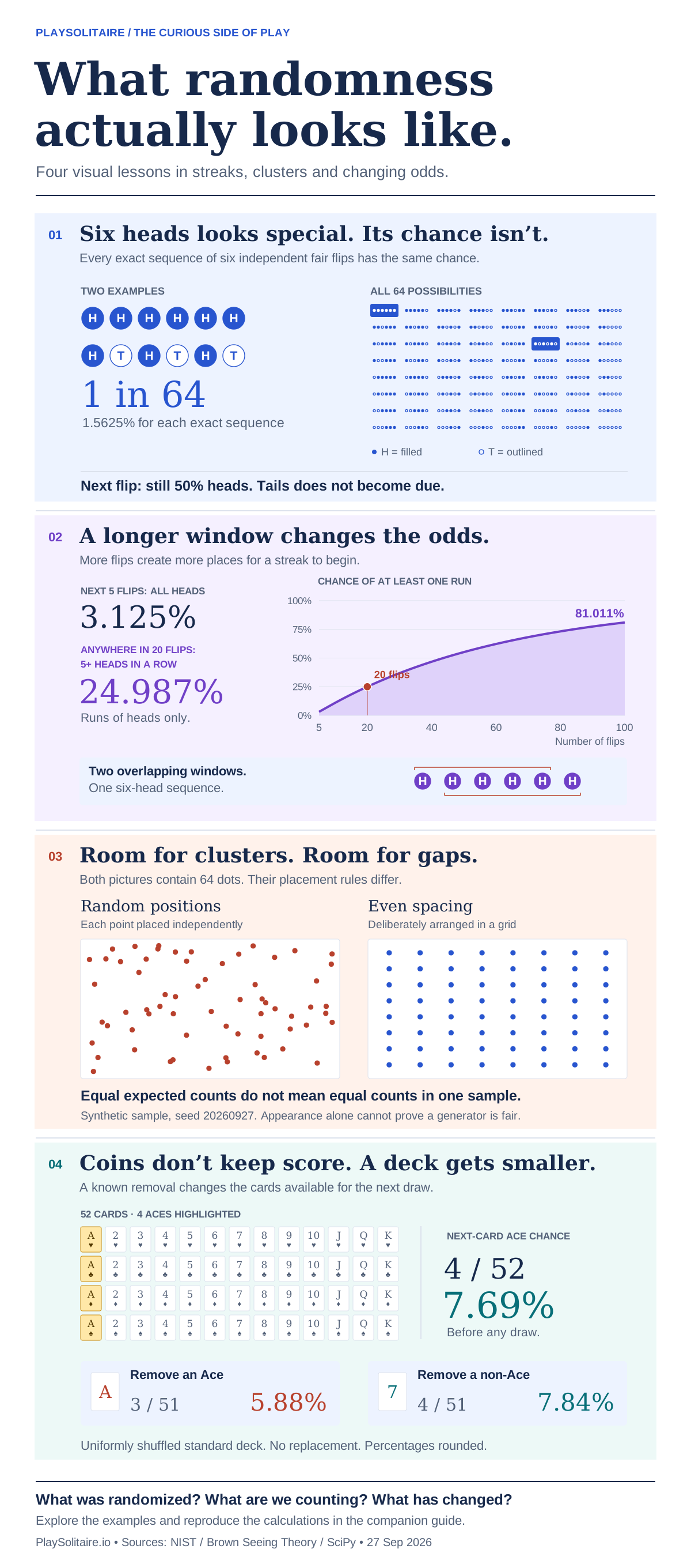
1 in 641.5625%
Each tile is one of the 64 possible outcomes. Filled dots = heads; outlined dots = tails.
The comparison changes when one side is a whole category. “All heads” contains one sequence. “Any mixture of heads and tails” contains 62. A larger category can be more likely even though every individual sequence has the same chance.
After six heads, the next independent fair flip is still 50% heads and 50% tails. Tails does not become due. The model contains no mechanism that compensates for what happened earlier.
That does not prove a real coin or generator is fair. It tells us what follows if the process is fair and independent. Evaluating an unknown process requires evidence about how it works.
A longer window gives a streak more places to appear
“Will the next five flips all be heads?” is different from “Will five heads appear in a row anywhere during the next twenty flips?” The first asks about one fixed block. The second allows a run to begin in several places.
The same streak becomes less surprising over time
3.125%Next 5 flips all heads
%5+ heads in a row within flips
Number of flips
At 20 flips, the probability is 24.987%, compared with 3.125% for the next five flips being all heads. At 100 flips, it rises to about 81.011%. A longer observation window changes how surprising a run is without changing the coin.
There is a catch: the possible starting positions overlap. A sequence of six heads contains two five-head windows. Adding their probabilities as though they were separate outcomes counts some sequences more than once.
We counted sequences containing no five-head run, then subtracted their share from one. An independent exhaustive check found that exactly 262,008 of the 1,048,576 twenty-flip sequences contain a qualifying run. The reproducible calculation is linked in the methodology.
Randomness leaves room for both clusters and gaps
Imagine placing 64 dots on a rectangle. Under a uniform random model, each dot gets an independently chosen horizontal and vertical coordinate. Every equal-area region has the same expected number of dots, but a particular sample need not divide them evenly.
Equal expectations. Unequal counts.
Random positions
One independent uniform sample
1–7 dots per region
Even spacing
An intentionally constructed grid
4 dots in every region
If we divide the placement area into 16 equal regions, each region has an expected count of 64 ÷ 16 = 4 dots. In the displayed random sample, the actual counts range from one to seven. In the constructed grid, every region contains exactly four.
Neither picture, by itself, establishes whether an unknown generator is fair. A cluster can occur under the random model; a tidy result can come from a rule that deliberately prevents clustering. The placement process is what makes the comparison meaningful.
A deck changes when a card is removed
Independent coin flips leave the next-flip probability unchanged. Drawing a card without replacing it changes the available population. A standard deck begins with four Aces among 52 cards, so the first-card chance of an Ace is 4/52, or about 7.69%.
What is left determines the next draw
Choose one known removal. Watch what remains.
4 Aces + 48 other cards
4 Aces ÷ 52 cards
All four Aces are still available. Choose a removal above to compare.
Before any draw
4 / 52
7.69%4 Aces among 52 cardsRemove an Ace
3 / 51
5.88%3 Aces among 51 cardsRemove a non-Ace
4 / 51
7.84%4 Aces among 51 cardsRemove an Ace and the next-card Ace probability falls to 3/51, about 5.88%. Remove any non-Ace and it rises to 4/51, about 7.84%. The remaining deck has changed, so the probability changes with it.
There is no contradiction between “tails is not due” and “the next Ace probability depends on which cards are gone.” Those statements describe different processes.
The population matters as much as the rule. Spider Solitaire 2 Suits uses 104 cards, with eight Aces across its two suits. Before any cards are dealt, that pack’s Ace share is also 1/13, but removing one Ace leaves 7/103, not 3/51. The one-deck calculation cannot simply be carried over after a removal; a probability for the stock during play must also account for cards already known elsewhere on the table.
Information matters too. In FreeCell, every card is dealt face up: the shuffled layout sets the puzzle, but there is no face-down stock to draw from. Uncertainty about how to solve that layout is a different problem from uncertainty about an unseen card. These examples describe information and card counts, not game win rates.
Three questions to ask before judging a random result
- What was randomized? A flip, a position or a deck order?
- What are we counting? One exact outcome, a larger category or a pattern anywhere in a session?
- What changed? The observation window, the information available or the remaining population?
Those questions identify the calculation that belongs to the problem. How orderly or disorderly the outcome looks is only a starting observation.
Methodology and sources
This is a mathematical explainer, not a survey or a study of player behavior. All examples and graphics were created for this article. The assumptions and data are provided so the results can be reproduced.
Coin sequences and streaks
The model uses fair, independent flips. For a run of five heads, we keep five integer counts of sequences with no qualifying run, indexed by trailing heads, zero through four. Start at [1, 0, 0, 0, 0]. Each flip updates them to [sum(counts), counts[0], counts[1], counts[2], counts[3]]. After n flips, subtract their sum from 2ⁿ and divide by 2ⁿ. The script verifies this recurrence against exhaustive enumeration.
Dot positions and card draws
The dot example uses Python’s pseudorandom generator with seed 20260927. Coordinates are independent uniform draws; points are not moved apart after generation. The data file also includes 11 further samples from consecutive seeds. Card examples assume a uniformly shuffled 52-card standard deck and one known removal without replacement.
- NIST/SEMATECH: Binomial distribution — background on fixed-probability success/failure counts. The consecutive-run calculation uses our separately verified recurrence.
- Brown University: Compound probability — background on counting outcomes and conditioning. No artwork or code reused.
- SciPy: Hypergeometric distribution — sampling without replacement. Our single-card examples use direct remaining-card counts.
Source pages checked September 27, 2026.
Download the graphics and calculations
Full visual summary (PNG)Editable artwork (SVG)Exact values and dot coordinatesStreak probabilities (CSV)Reproducible Python script